Modern computer vision applications rely on live video capturing. Until now we were discussing only single image processing as a field of computer vision. Now, it’s time to introduce another dimension in our computer vision applications, time. Videos from live cameras can be used for so many purposes such as security, quick digital measurement, traffic regulation and others. So let’s see how we can use our knowledge from image processing and apply it to video processing.
This bundle of e-books is specially crafted for beginners.
Everything from Python basics to the deployment of Machine Learning algorithms to production in one place.
Become a Machine Learning Superhero TODAY!
1. Video Capturing Setup Using OpenCV
Before we dive into any video processing and some further explanation on how you can apply image processing knowledge into video applications we should first set up everything that we need for live recording. In this article we are going to use an example video from the internet, but we will show you how to use a web camera from your machine. So without any further ados let’s dive into code.
1.1 Setup
Firstly we need to understand what video is and how it’s related to the image. Videos are just image sequences where images change really fast. So if you want to do some transformation on a video you need to apply the same transformation to every image in that sequence. Those images are called frames. In order to simulate video, we’ll need to make an infinite loop that displays frames very fast. Using OpenCV, it’s going to look something like this:
import cv2

recording = cv2.VideoCapture(0)

while True:

   ret, frame = recording.read() #ret is True or False value depending on whether we successfully got an image from recording
   cv2.imshow('Frame', frame)

   if cv2.waitKey(1) == ord('x'):
       break

cv2.destroyAllWindows()
As we can see we’ve created an object recording of class VideoCapture. Argument zero tells VideoCapture that we want to use a web camera from our machine. If you have multiple cameras on your machine you can access them using numbers 1, 2, 3 and so on. As we said we’re not going to use our web camera to make recordings, but we’ll use an example video from the internet. We just need to put that video path instead of a zero:
recording = cv2.VideoCapture('test.mp4')We are using an infinite loop to read and display each frame from our recording. Variable ret is a boolean value, True or False depending on whether we successfully got an image from recording. Each millisecond we’ll check if the ‘x’ key is pressed and that will break our loop. Also when we break the loop we’ll need to close all the windows.
2. Building a Document Scanner with OpenCV
Now that we know how to process videos as single frames, let’s build a document scanner that will pick up video footage of a document from any given angle, warp the perspective and performs image segmentation so it ends up looking something like this.

2.1 Load Video
We are going to use this video of a document on a table. Our plan is to perform edge detection, find the biggest contour that will represent the shape of the document, then warp the perspective and lastly perform Thresholding.
We’re going to be using the following libraries:
import numpy as np
import cv2
import imutils
Let’s now load the video and see what it looks like.
cap = cv2.VideoCapture('video-1657993036.mp4')
if cap.isOpened() == False:
   print("Error opening the video")

while cap.isOpened():
   ret, frame = cap.read()
   frame = cv2.resize(frame, (812, 812))
   cv2.imshow('frame', frame)

cap.release()
cv2.destroyAllWindows()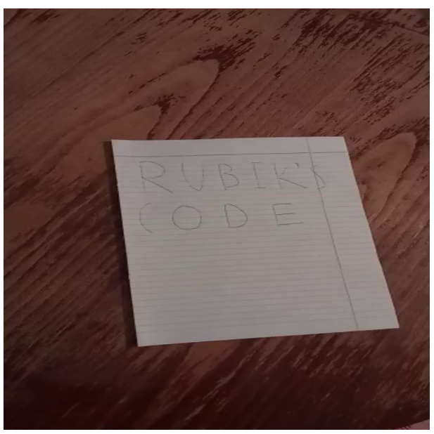
2.2 Detect Edges
The frame size was unnecessarily big so we performed resizing using cv2.resize and set it to an 812×812 frame.
To find the edges of an image we first need to convert it to a gray image, then we want to apply the noise (blur) so we get rid of unnecessary contours. After that is done we want to apply Canny edge detection.
gray_frame = cv2.cvtColor(frame, cv2.COLOR_BGR2GRAY)
img_blurred = cv2.GaussianBlur(gray_frame, (5, 5), 1)
edge_image_blurred = cv2.Canny(img_blurred, 60, 180)
cv2.imshow("Edge image”, edge_image_blurred)
The result is as following:

2.3 Image Dilation
The next thing to do is find contours, but before we do that we should discuss one problem that might pop up. Since we’re processing a video that consists of multiple frames, not every frame is going to be shot from the same angle and therefore we will encounter deviation when it comes to lighting and other stuff.
What that does is it doesn’t always perfectly find the contour of a document that we want, in other words, there might be missing pixels and that would result in our job not being properly done.
To solve that problem we will apply something called image dilation. In image processing, the said method adds pixels to the boundaries of objects. The opposite of dilation is erosion.
kernel = np.ones((5, 5))
imgDil = cv2.dilate(edge_image_blurred, kernel, iterations=2)
cv2.imshow('ImgDilated', imgDil)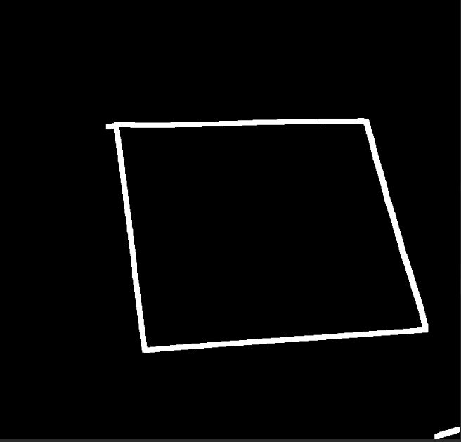
2.4 Contour Detection
The difference is quite noticeable.
Now that we are all set and done, let’s perform contour detection.
key_points = cv2.findContours(imgErod, cv2.RETR_EXTERNAL, cv2.CHAIN_APPROX_SIMPLE)
contours = imutils.grab_contours(key_points)
cv2.drawContours(frame, contours, -1, (0, 255, 0), 2)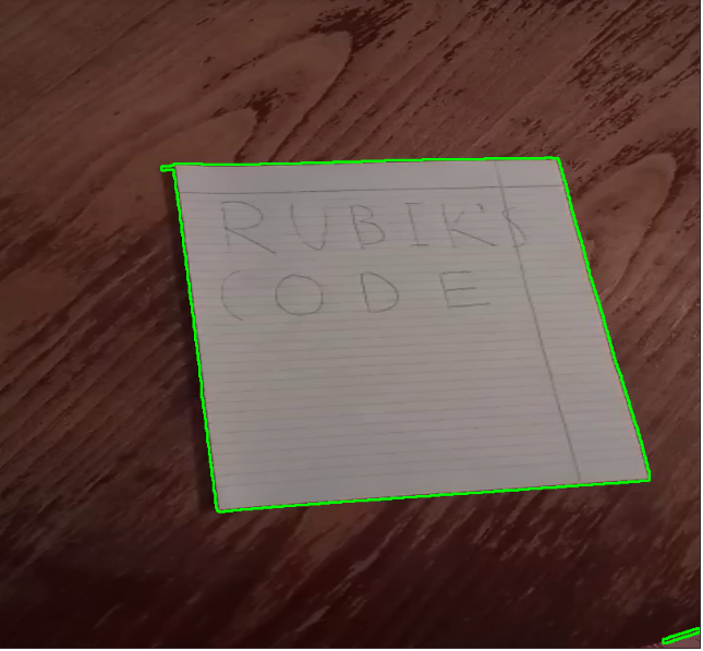
We now want to extract the biggest contour as it will represent the document boundaries. To do that we are going to go through all contours, and pick those with an area bigger than 10000. That number was chosen experimentally just to get rid of obviously small contours that cannot fit the description of a paper. After that, we want to find the polygon-like contours that can be formed with 4 points, which will represent a paper.
biggest_contour = np.array([])
for contour in contours:
   area = cv2.contourArea(contour)
   if area > 10000:
       perimeter = cv2.arcLength(contour, True)
       approximation = cv2.approxPolyDP(contour, 0.05 * perimeter, True)
       if len(approximation) == 4:
           biggest_contour = approximation
Biggest_contour variable will be an array that holds 4 points that resemble a polygon shape that fits the description of a paper on a table.
Let’s draw those 4 points and see if we got it right.
if biggest_contour.size != 0:
   cv2.drawContours(frame, biggest_contour, -1, (0, 255, 0), 15)
2.5 Perspective Wrap
As we can see, everything is going according to plan so far.
Now that we have those 4 points, we want to perform a perspective warp. If you’re confused with the parameters check our article on geometric transformations with openCv, in which we’ve covered these things in depth.
if biggest_contour.size != 0:
   cv2.drawContours(frame, biggest_contour, -1, (0, 255, 0), 20)

   pts1 = np.float32(biggest_contour)
   pts2 = np.float32([[0, 0], [0, 512], [512, 512], [512, 0]])
   P = cv2.getPerspectiveTransform(pts1, pts2)
   image_warped = cv2.warpPerspective(frame, P, (512, 512))

cv2.imshow('Warped image', image_warped)
2.6 Treshold
All that is left to do is perform thresholding on our image.
Here we can use global thresholding as the image appears to have a bimodal histogram, but usually when scanning documents we would want to apply adaptive thresholding, so we’re going to go with the norm. We should note that we warped the gray image since thresholding only works on gray-scale images.
if biggest_contour.size != 0:
   cv2.drawContours(frame, biggest_contour, -1, (0, 255, 0), 20)
   pts1 = np.float32(biggest_contour)
   pts2 = np.float32([[812, 0], [0, 0], [0, 812], [812, 812]])
   P = cv2.getPerspectiveTransform(pts1, pts2)
   image_warped = cv2.warpPerspective(gray_frame, P, (812, 812))
   binary_image = cv2.adaptiveThreshold(image_warped, 255, cv2.ADAPTIVE_THRESH_GAUSSIAN_C, cv2.THRESH_BINARY, 71,                               9)
   cv2.imshow('frame', binary_image)
Conclusion
With this article, we will end this small but useful series. We’ve learned some basic concepts of image processing, which are usually just a step in the whole computer vision process. We hope that you had fun following these tutorials and that you stick around for our future tutorials and projects.
Authors
Stefan Nidzovic
Author at Rubik's Code
Stefan Nidzovic is a student at Faculty of Technical Science, at University of Novi Sad. More precisely, department of biomedical engineering, focusing mostly on applying the knowledge of computer vision and machine learning in medicine. He is also a member of “Creative Engineering Center”, where he works on various projects, mostly in computer vision.

Milos Marinkovic
Author at Rubik's Code
Miloš Marinković is a student of Biomedical Engineering, at the Faculty of Technical Sciences, University of Novi Sad. Before he enrolled at the university, Miloš graduated from the gymnasium “Jovan Jovanović Zmaj” in 2019 in Novi Sad. Currently he is a member of “Creative Engineering Center”, where he was involved in a couple of image processing and embedded electronic projects. Also, Miloš works as an intern at BioSense Institute in Novi Sad, on projects which include bioinformatics, DNA sequence analysis and machine learning. When he was younger he was a member of the Serbian judo national team and he holds the black belt in judo.


A very interesting and well written article. I want to try this out also on the Raspberry Pi.
But howcan one access a WebCam And/or the Pi camera on the Raspberry pi?